Country Specific – Denmark
Quick Facts about the Danish model (DHM)
| Cell Size | 40x40 cm |
| Coordinate System | ETRS89 / UTM 32N |
| Vertical Reference | DVR90 |
| Flight Years | 2018–2022 |
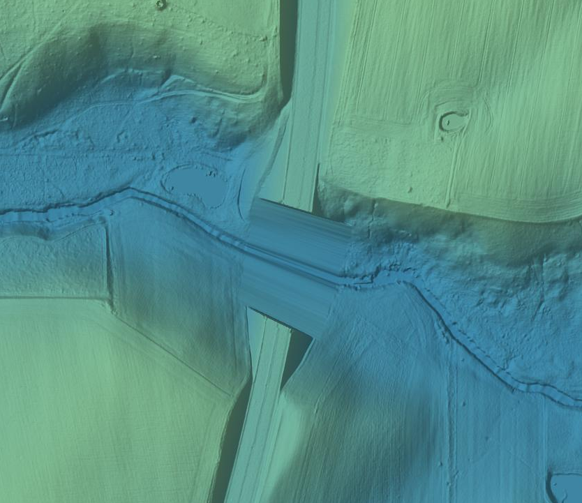
Our Danish elevation model is based on the official Danish elevation model (also known as DHM) produced by the Agency for Data Supply and Infrastructure (SDFI). Since 2018, SDFI updates the elevation model in partial increments of about a fifth of the country every year. The model has a horizontal resolution of 0.4 m and was released for the first time in this resolution in 2015, improving upon the previous model from 2007, which had a resolution of 1.6 m. The model is available in SCALGO Live under the name Terrain (Terræn). There are a couple of different variants of the model available.
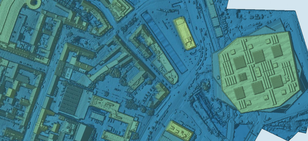
Terrain/Buildings (Terræn/Bygninger): This is the raw model enriched with building footprints from the national GeoDanmark data set. For each GeoDanmark building footprint, we've raised the elevation of the cells there are inside the buildings with 10 m, relative to the highest elevation value of the original terrain model.
Terrain/Buildings/Rain (Terræn/Bygninger/Regn) and Terrain/Buildings/Sea (Terræn/Bygninger/Hav): Both models are derived from the Terrain/Buildings model and include the set of hydrological corrections from GeoDanmark.
Terrain/Buildings/Rain includes the corrections made for modeling water flowing downstream on the terrain, e.g., water from rain events. Terrain/Buildings/Sea is targeted for modeling flooding from sea. The main difference between the two models is infrastructure like sluices, and whether they are open or closed.
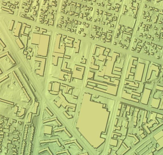
Surface (Overflade): This is the Digital Surface Model (DSM) version of the DHM. In this model houses, vegetation etc. is preserved in the elevation model.
Sources: A source layer, showing the acquisition year of the data, is available by clicking the gear icon next to an elevation layer and selecting the "Source" ("Kilde") tab, and then "Show source information" ("Vis kildedata"). Use it to figure out how old the data is for your project area. You can use the point query tool to get the acquisition year for a particular area.

Terrain (2015) (Terræn (2015)):
This is a historical version of DHM, released in 2015 based on scans from 2014-2015. It was the first model released by SDFI with a resolution of 0.4 m.
Surface (2015) (Overflade (2015)):
This is the Digital Surface Model (DSM) version of DHM from 2015.
Terrain (2007) (Terræn (2007)):
This is an older model of Denmark released in 2007 based on scans from 2005-2007. It has a horizontal resolution of 1.6 m.
Surface (2007) (Overflade (2007)):
This is the Digital Surface Model (DSM) version of DHM from 2007.
Terrain (QuickDHM) (Terræn (QuickDHM)):
This is a temporary version of DHM with the newest available data from SDFI. Is have not been quality checked and errors and missing data occurs. It has a horizontal resolution of 0.4 m.
Surface (QuickDHM) (Overflade (QuickDHM)):
This is the Digital Surface Model (DSM) version of QuickDHM.
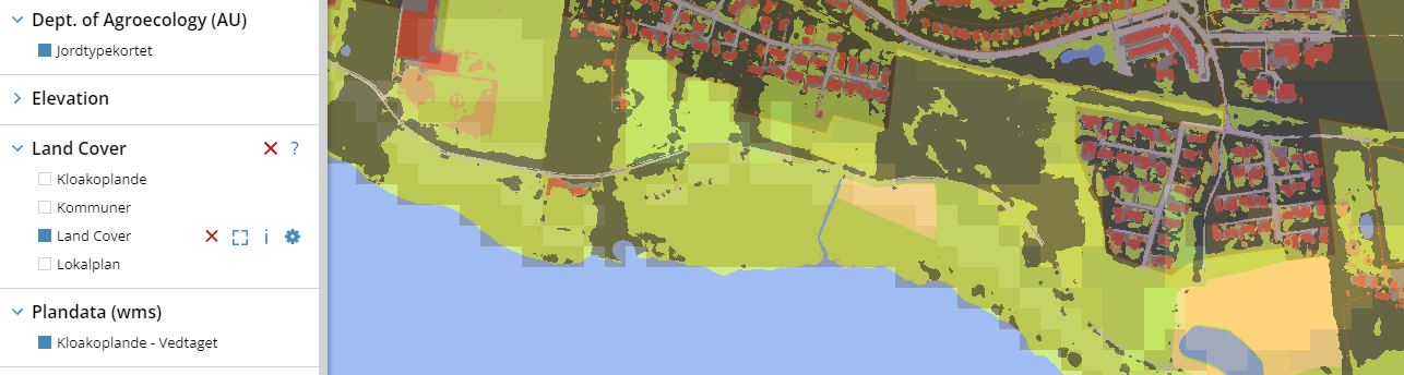
Land cover (Arealdække)
The land cover map in SCALGO Live is produced by SCALGO based on machine learning techniques at a resolution of 20 cm. It is available as a standalone layer in the Land Cover category in the library.
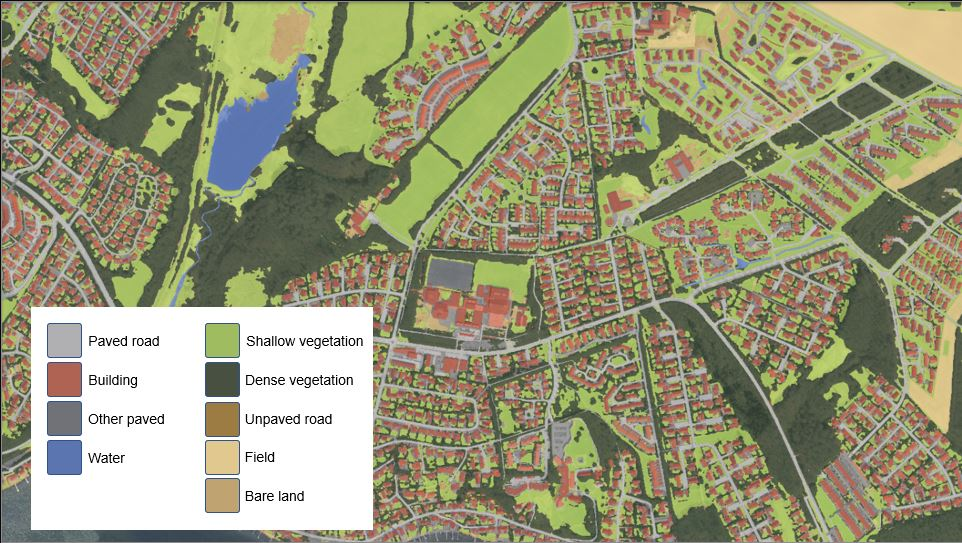
The land cover map segments the country into 9 different classes as seen in the above graphic. When downloaded as a raster, the categories have the following numerical encoding: 1 for bare land, 2 for water, 3 for other paved, 6 for shallow vegetation, 7 for dense vegetation, 8 for farmland, 9 for paved road, 10 for unpaved road, and 16 for building.
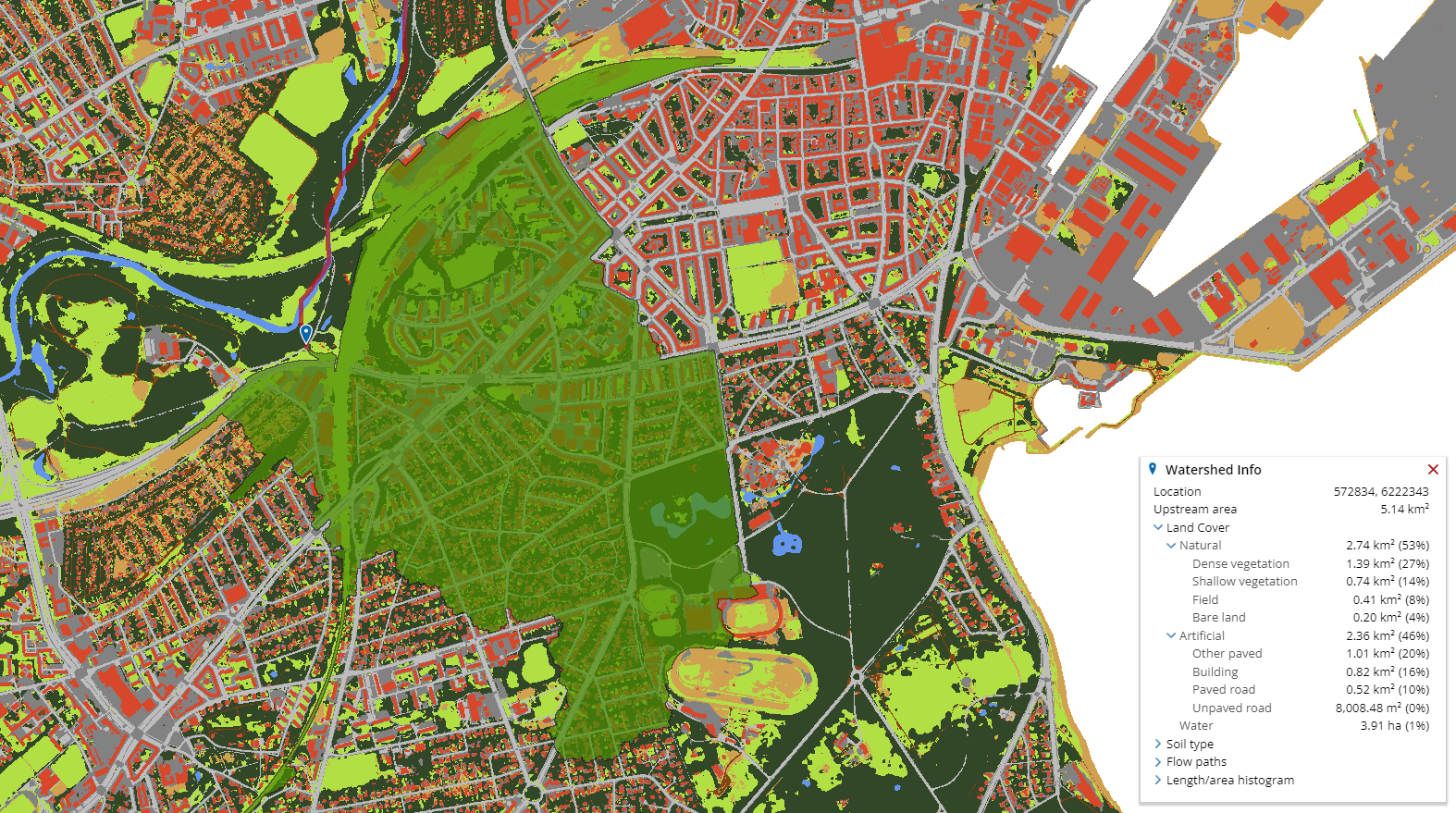
Watershed queries
When you perform a watershed query you can see the land cover distribution of the watershed.
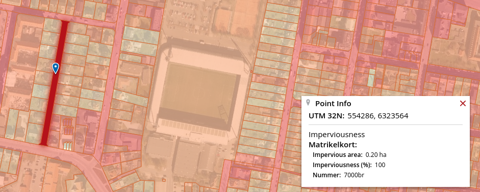
Annotated administrative regions
We have annotated a number of datasets, including the cadastral parcels, sewer catchments, planning zones as well as municipal regions with information about land cover. You can find those layers in the Land Cover category alongside the land cover map itself. For each region in those data sets we have added a field that provides the total impervious area in the region, as well as the ratio of imperviousness to perviousness in the region.
Soil type (Jordtypekortet)
SCALGO Live uses Jordtypekortet (30 m resolution) from the Department of Agroecology at Aarhus University, both for watershed queries and in the Flash Flood Map. In watershed queries it is available as aggregate information about the composition of soil types in a given watershed, and in the Flash Flood Map it forms the basis for determining rates of infiltration from pervious cells when enabling infiltration and drainage. Jordtypekortet classifies the topmost soil layer of Denmark into types based on soil samples taken mainly from farmland, interpolated to cover the entire country in a 30.4 m resolution grid. We refer to a memo (in Danish) published by the Danish Centre for Food and Agriculture for more information on the soil type map.
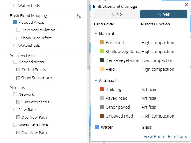
Infiltration and drainage to sewers
The Flash Flood Map supports the use of runoff functions to specify the runoff generated from each cell as a function of the rain depth. In Denmark we have produced a national Flash Flood Map where we use runoff functions to include infiltration and drainage to sewers in the model. When you enable infiltration and drainage in the Flash Flood Map, the infiltration at a cell is determined by the cell’s land cover class as well as its soil type (in pervious areas) and sewer map status (in impervious areas).
In impervious areas, if a cell is in an area that has a combined sewer system (treating both surface water and wastewater), then an amount of rain corresponding to a 10-year event is subtracted as initial loss; if the cell is in an area with a dedicated surface water system, a 5-year event is subtracted as initial loss. Other impervious areas use the glass model with no initial loss.
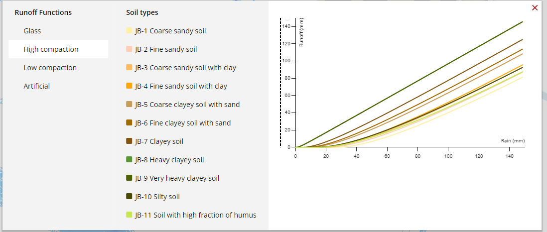
In natural areas, dense vegetation areas are assumed to have loose soil, while shallow vegetation and bare land areas are assumed to have compacted soil. Each soil type in the soil type map has a CN curve for both compact and loose conditions.
For more information about the Flash Flood Map with infiltration and drainage, including information about parameter settings and CN-curve numbers, we refer to our in-depth white-paper.
To view the runoff functions used for individual soil types, click “View Runoff Functions” in the infiltration and drainage popup.
If you want to investigate the sewer type mapping and the soil type data used in the computation you can find them both in the library.