Country Specific – Sweden
Quick Facts Markhöjdmodell
| Cell Size | 1x1 m |
| Coordinate System | SWEREF99 TM |
| Vertical Reference | RH 2000 |
| Flight Years | 2009–present |
Elevation models
Our main elevation model of Sweden is based primarily on Lantmäteriet's Markhöjdmodell Nedladdning, grid 1+ with a grid resolution of 1x1 meter. The ground data for this model was acquired by airborne LIDAR scans from 2009 and forward through two projects: Laserdata Nedladdning, NH and Laserdata Nedladdning, skog. Since Laserdata Skog is also available as a more regularly updated raw point cloud, we publish an additional elevation model based only on this data. More information on this model and the differences with Markhöjdmodell can be found below.
We strive to keep our models up to date with the latest sources.
In order to use an elevation model for hydrological analysis such as watershed and flow accumulation computations, three primary conditions should be met:
- The upstream area of any river should be covered by the elevation model.
- Structures on top of the terrain should only be present in case they actually block water from flowing under or through them.
- Structures transferring water below the terrain surface should be taken into account.
Below, we discuss how we process the model to fulfil these conditions as well as possible.
Extensions
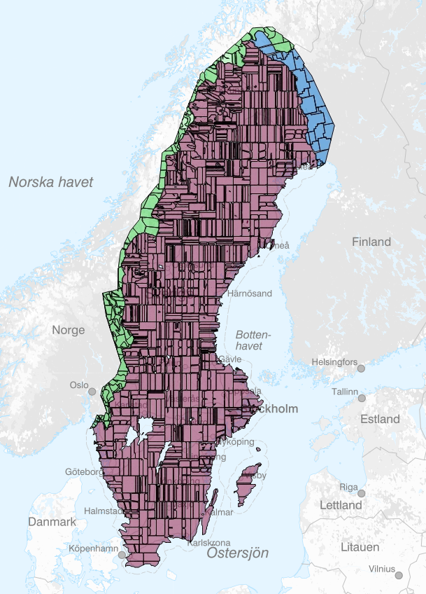
In order to cover the upstream areas of all rivers in Sweden, we have extended the Markhöjdmodell in the following areas:
- To cover the upstream area of Torneälven in Finland, we include data from the national Finnish 2-meter model from Lantmäteriverket (blue in the figure below), and, in a few small areas, Lantmäteriverket's Höjdmodell 10 m.
- To cover upstream areas in Norway, we include data from the Norwegian national detailed elevation model (NDH) from Kartverket (green areas in the figure below) as well as Kartverket's DTM 10 (light green). This last model is based on varying sources such as contour lines and peak elevations.
A full overview of which data source is used for which part of the model is available clicking the gear icon next to an elevation layer, selecting the "Source" tab, and "Show source information". Use point query to see more details for individual areas as provided by Lantmäteriet. Multiple styles are available for this layer to colour sources by e.g. collection date.
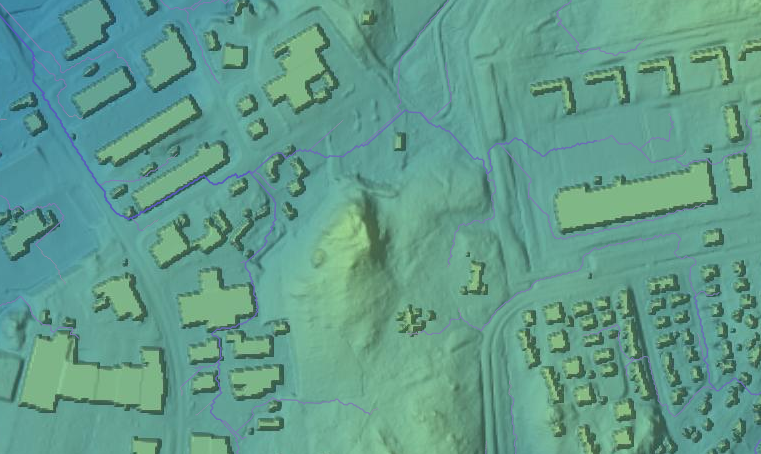
Buildings
Buildings have been removed from the terrain model during construction. When computing water flow paths, more realistic results are generally obtained when the elevation model does include buildings so that water can be simulated to flow around them. In SCALGO Live, we accomplish this by adding buildings back into the model using a data set of building footprints where we raise all grid cells covered by a building to a height of 10 m above the highest terrain point within the building footprint. This model is called Terrain/Buildings and is the basis for all nationwide hydrological computations.
The building footprint data set used is Lantmäteriet's Byggnad Nedladdning, vektor. This layer can be shown and downloaded individually and it can be found in the Lantmäteriet category in the Library.
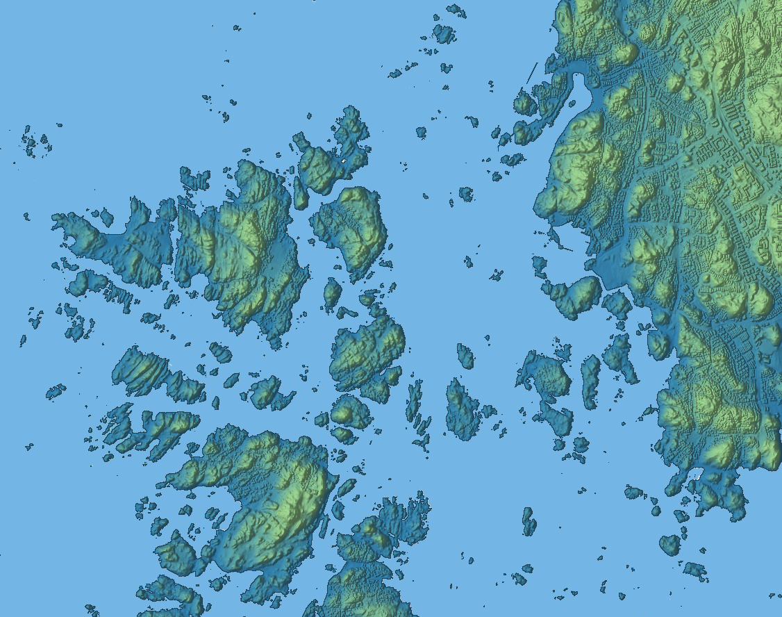
Coastline
Since the elevation of grid cells in the sea around Sweden is not consistent in the source data, we have masked out these cells using the Shoreline layer in Lantmäteriet's Hydrografi Nedladdning (also available as a layer in the Hydrografi category in SCALGO Live).
Bridges, underpasses and hydrological corrections
Major bridges and underpasses have generally been removed from Lantmäteriet's Markhöjdmodell, but for
many smaller bridges and underpasses additional hydrological
corrections that allow water to flow through such structures are necessary. SCALGO Live in Sweden includes two nationwide hydrological correction sets, a conservative set of corrections based on authoritative data sources and a comprehensive set based on machine learning. They are both available under the Hydrological Corrections category in the Library.
The national analyses use only the conservative corrections, and workspaces created using the predefined "Flash Flood Map" or "Sea-Level Rise" buttons also include the conservative corrections by default. The comprehensive corrections can optionally be included in the workspace afterwards through the workspace Actions tab by clicking Import corrections. Note that you should then also include the conservative corrections if they are not already in your workspace. If you create a workspace through any other means than the predefined buttons (e.g. if you upload your own model), you can include corrections in that workspace in the same manner, they will not be included automatically.
Conservative corrections
The conservative corrections have been generated primarily based on the network in Lantmäteriet's Hydrografi Nedladdning product. Corrections have been generated at locations where the network intersect roads, railroads, dams, weirs, or buildings, as well as at invisible river sections where the river e.g. runs through a longer covered/piped area. Each correction thus follows a line in the river or road network, with end points adjusted to match the elevation model as well as possible. In places where the elevation model is already hydrologically corrected (e.g. at large bridges), corrections are not generated. Furthermore we have included corrections at road underpasses and places where roads intersect buildings, as well as a few of the machine-learned corrections from the comprehensive corrections in the places where those corrections align well with the river network.
This data set is machine-generated, so some errors should be expected. However, since we only include corrections along known river lines, we believe it to be conservative in terms of water flow.
Comprehensive corrections
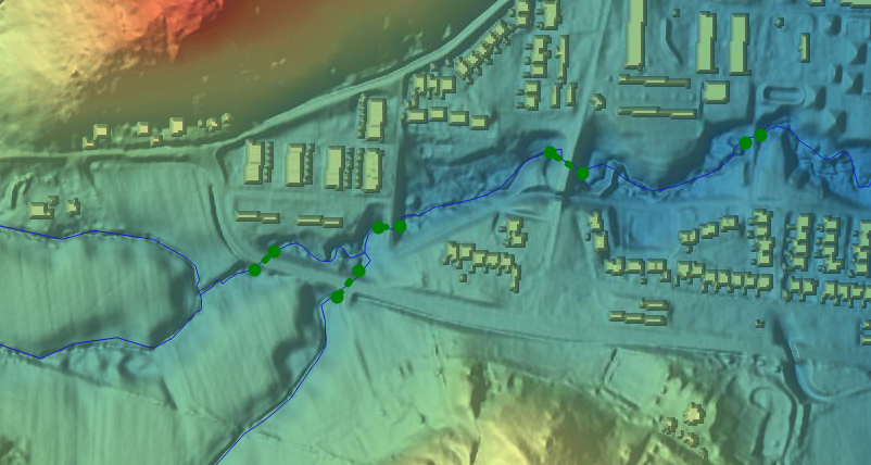
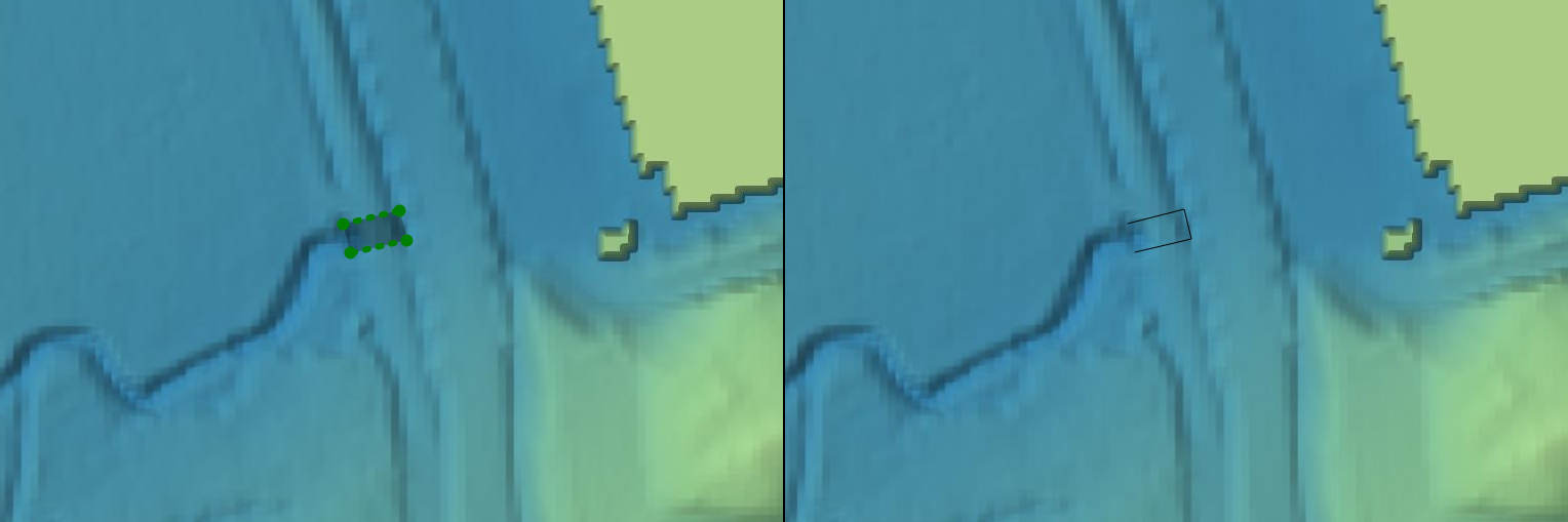
This correction set is generated using a machine-learning model trained on a large number of known locations of culverts, bridges, etc. The model was then used to predict locations for corrections in Sweden using Markhöjdmodell. The result is a correction set with unprecedented coverage of especially smaller culverts and underpasses. The data has not been manually verified and is likely to contain spurious corrections and miss others. The comprehensive set of corrections is not included in our national analyses or in workspaces by default. However, we believe it could save our users a lot of time compared to manually identifying and entering corrections for areas away from main rivers. Some key notes to keep in mind regarding the comprehensive set of corrections:
- Corrections are represented as areas instead of lines, where water can flow between the two ends (see screenshots below).
- There are more false positives in certain areas.
- Comprehensive corrections that intersect conservative corrections have been removed to prevent duplicates.
Quick Facts Laserdata Skog
| Point Density | 1-2 points/m2 |
| Coordinate System | SWEREF99 TM |
| Vertical Reference | RH 2000 |
| Flight Years | 2018– |
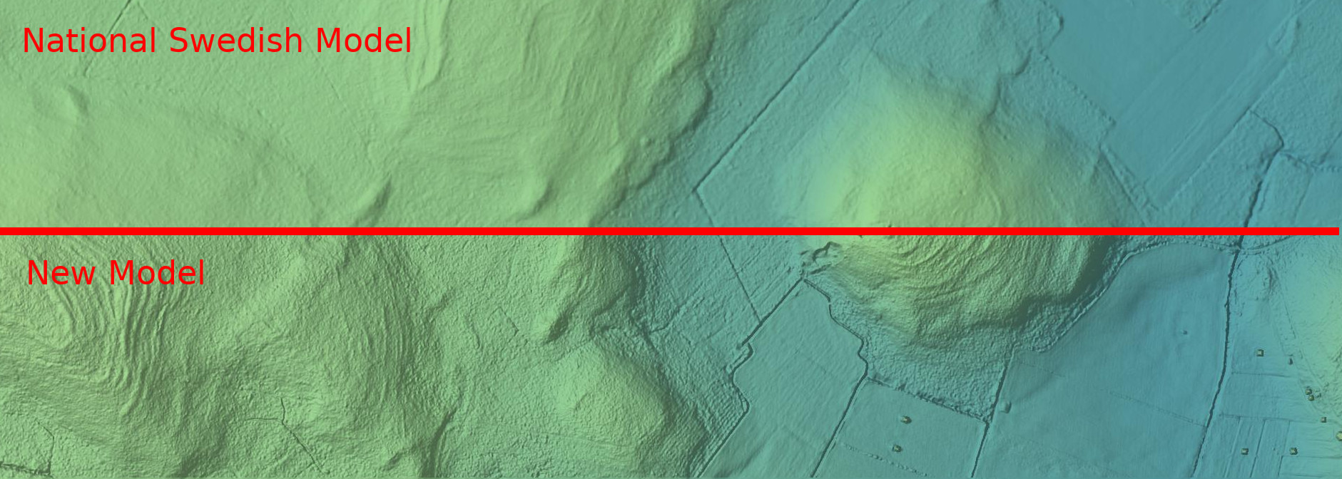
Laserdata Skog
Since fall 2018, Lantmäteriet has published a LIDAR-based elevation dataset called Laserdata Skog. The main differences between this data set and Markhöjdmodell Nedladdning, grid 1+ are:
- Laserdata Skog is more up-to-date (continuously updated as new data is released).
- Laserdata Skog only contains data with a high point density (1-2 points per square meter), where Markhöjdmodell also includes older, lower resolution data from the Laserdata NH project.
- Laserdata Skog does not yet cover all of Sweden (see Planer och Utfall, Långsiktig skanningsplan).
- Laserdata Skog is not published as a raster DEM by Lantmäteriet, which means that bridges are not removed and lakes are not flattened.
- Laserdata Skog is open data (CC0).
SCALGO Live includes a 1x1 meter raster DEM based on the ground-classified point cloud as well as a model with buildings raised using building footprints from Lantmäteriet's Byggnad Nedladdning, vektor data set. The model will be updated regularly to include new data published by Lantmäteriet. You can visualize the elevation model as well as download it and use it as basis for workspaces. If you want to use it in a workspace, use existing model and click the pencil next to the elevation model in the dock after selecting your workspace region.
Land cover
The land cover map in SCALGO Live is produced by SCALGO based on machine learning techniques at a resolution of 20 cm. It is available as a standalone layer in the Land Cover category in the library.
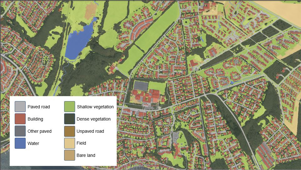
The land cover map segments the country into 10 different classes. When downloaded as a raster, the categories have the following numerical encoding: 1 for bare land, 2 for water, 3 for other paved, 6 for shallow vegetation, 7 for dense vegetation, 8 for farmland, 9 for paved road, 10 for unpaved road, 15 for bare rock, and 16 for building.
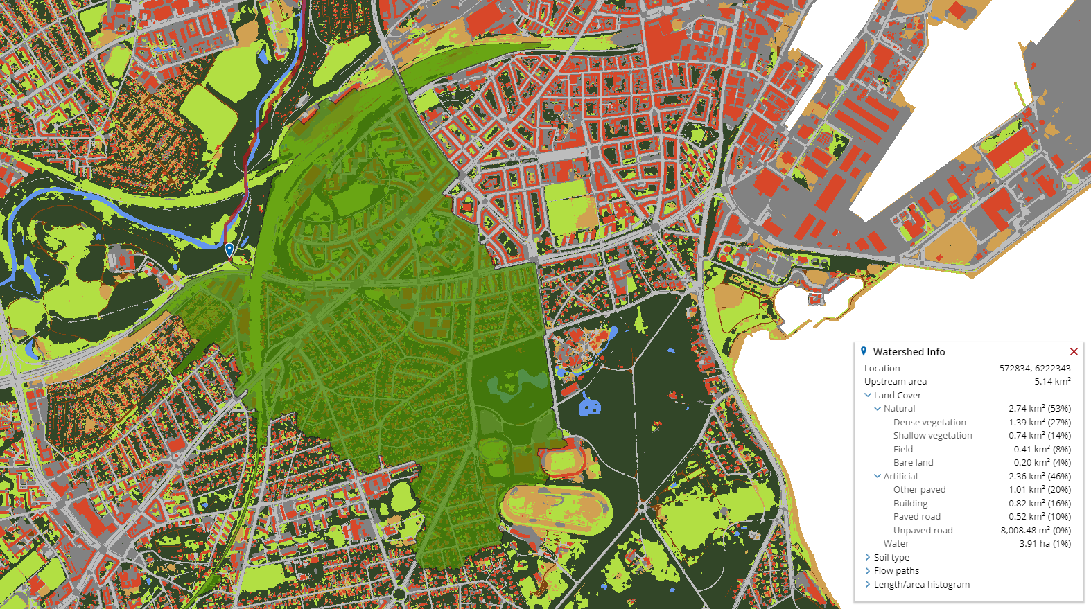
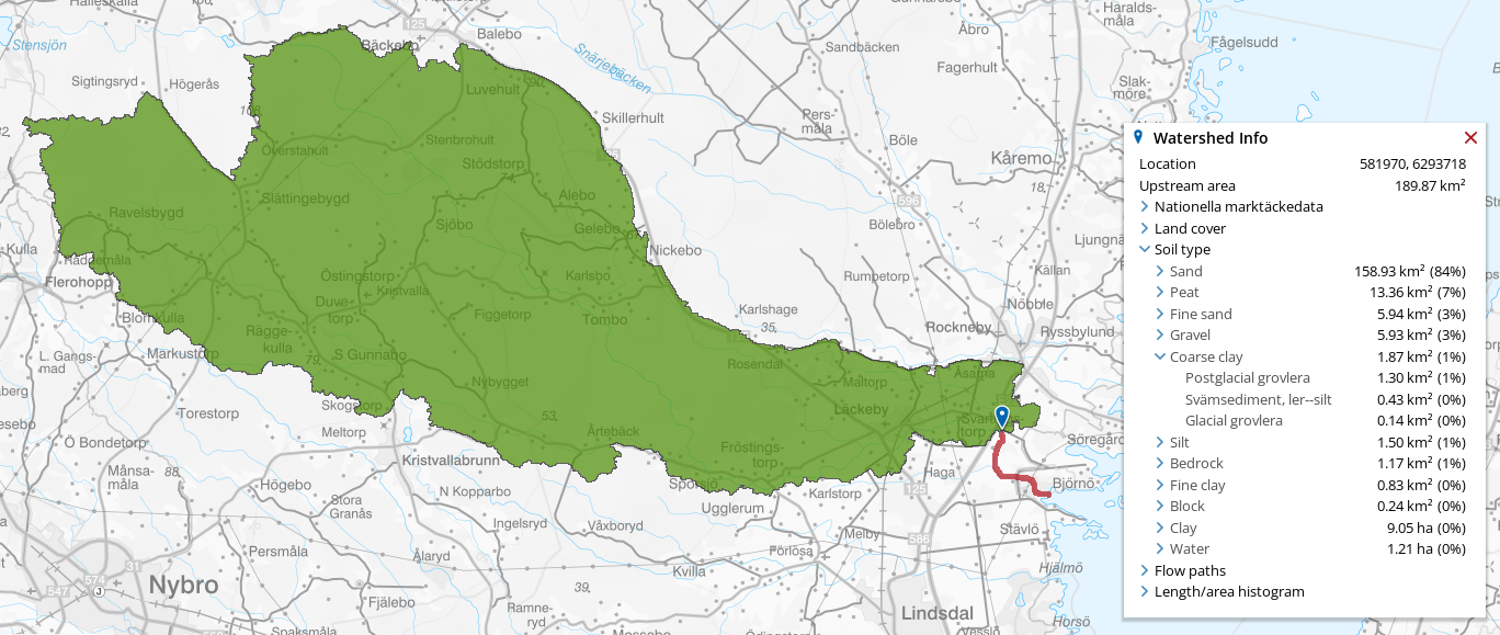
Watershed queries
When you perform a watershed query you can see the land cover distribution of the watershed.
Annotated administrative regions
We have annotated a number of datasets, including the cadastral parcels and urban zones with information about land cover. You can find those layers in the Land Cover category alongside the land cover map itself. For each region in those data sets we have added a field that provides the total impervious area in the region, as well as the ratio of imperviousness to perviousness in the region.
Nationella Marktäckedata
SCALGO Live shows coverage statistics based on Nationella Marktäckedata (NMD) from Naturvårdsverket for watershed queries. Nationella Marktäckedata is a mapping of land cover in Sweden at 10 m resolution, and is based on a combination of satellite data with information from the national laser scanning. To a lesser extent, it incorporates geographic data from various government authorities. We refer to Naturvårdsverket for more information about the Nationella Marktäckedata.
Soil type (Jordarter)
SCALGO Live uses superficial deposits data from the Geological Survey of Sweden (SGU) for watershed soil type queries. We combine five soil type datasets, GE.Jordarter 1:25 000 – 1:100 000, GE.Jordarter 1:200 000, GE.Jordarter 1:250 000, GE.Jordarter 1:750 000 and GE.Jordarter 1:1 000 000.
Jordarter 1:25 000 – 1:100 000 is used by default, but it does not cover all of Sweden. Where Jordarter 1:25 000 – 1:100 000 is not available, we have used the next best available soil type map for an area.
The different soil type maps have similar categorizations of soil types. If a category is the same in two or more datasets, it will be merged into one category, e.g. "Lera–silt" (clay–silt) is present in all datasets. If a category is unique, then it will remain intact also after combining the soil type maps. Jordarter 1:25 000 – 1:100 000 typically has finer categorization and unique categories, such as "Glacial finlera" (Glacial fine clay). The combined map is available as the "Jordarter - landstäckande" layer in the SGU category.
There are many soil type categories, and they have therefore been grouped to simplify presentation, see the figure below. Each group (such as “Coarse clay”), lists the sum of the areas of all soil types in that group found in a watershed. Information about each individual soil type is shown as a subcategory.
The soil type categories are the same as for the Flash Flood Map with infiltration and sewers, we refer to the whitepaper referenced in the next section for more information about the categorization. The "Reclassified soil types" layer in the SGU category shows the result of the grouping.
Infiltration and drainage to sewers
The Flash Flood Map supports the use of runoff functions to specify the runoff generated from each cell as a function of the rain depth. In Sweden we have produced a national Flash Flood Map where we use runoff functions to include infiltration and drainage to sewers in the model. When you enable infiltration and drainage in the Flash Flood Map, the infiltration at a cell is determined by the cell’s land cover class as well as its soil type (in pervious areas) and sewer map status (in impervious areas).
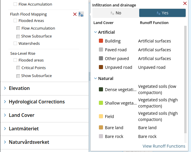
For artificial surfaces, we distinguish between those that are expected to be served by sewer systems, and those that are not. We assume that all artificial surfaces within an urban zone (defined using the dataset Tätorter from SCB) are connected to a sewer system, while all those outside these zones are not. For the artificial surfaces connected to a sewer system, we calculate the runoff as the rainfall minus the expected capacity of the sewer system, defined by a CN-p curve. For all other artificial surfaces we assume 100% runoff.
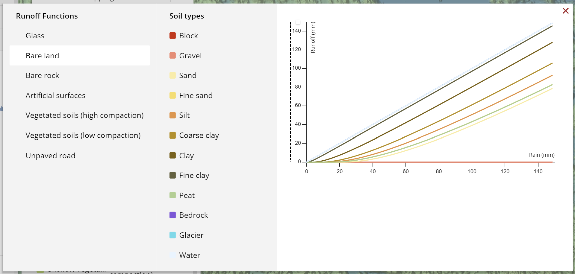
For natural surfaces, we generally calculate the runoff as the rainfall minus the infiltration, using CN-p curves. The infiltration is assessed based on the soil type and the expected degree of compaction of the soil type, which is assessed based on the land cover class.
For more information about the Flash Flood Map with infiltration and drainage, including information about parameter settings and CN-curve numbers, we refer to our in-depth whitepaper.
To view the runoff functions used for individual soil types, click “View Runoff Functions” in the infiltration and drainage popup.
Note that the inputs mentioned above are available as layers in SCALGO Live:
- Land Cover / Land Cover
- SGU / Reclassified soil types
- Land Cover / Tätorter