About – What's new
National hydrological corrections and updated local data for Finland
We have released a significant upgrade to the Finnish model in SCALGO Live. We have included new elevation data for Helsinki and Lahti, and we have produced hydrological corrections for the entire country which we have used in the analysis.
Hydrological corrections
Hydrological corrections make it possible to model water that flows through supposed obstacles in the elevation model that actually allow water to flow in reality. For instance, when a stream crosses a road under a bridge, the elevation model could make it look like there is a blockade since the space under the bridge is not represented.
We treat hydrological corrections as logical structures that allow water to flow from one end to the other, they typically do not alter the elevation model itself. Thus, waterways can cross in SCALGO Live — a very powerful feature. For instance, water can flow on top of a bridge in the direction of the road, and at the same time a river can cross the road under the bridge in a different direction. Hydrological corrections have infinite transport capacity, we do not model flooding from e.g. under-dimensioned culverts and bridge openings.
When you create a workspace, the hydrological corrections are included automatically, unless you create a model from a custom DEM or through the "Existing model" feature — in that case you can choose to import corrections directly from the workspace itself.
Updated elevation data for Helsinki and Lahti
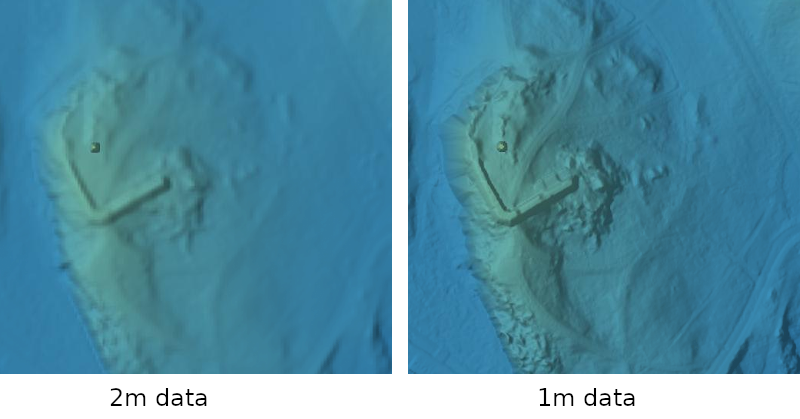
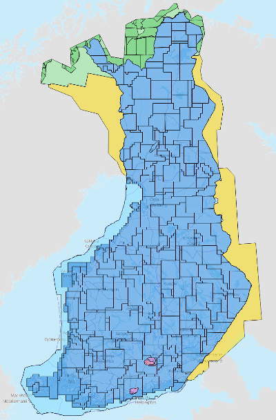
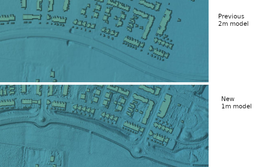
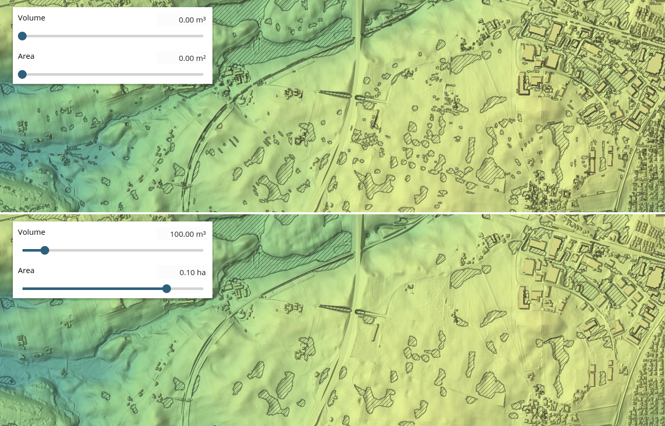
For the areas around Helsinki and Lahti, we now use elevation models with a horizontal resolution of 1 meter made available for SCALGO Live users by the respective municipalities. This provides a substantial lift in data quality for users in those areas. In order to incorporate these models, we now represent the whole country in a 1 m model instead of a 2 m model. This also holds for workspaces created from this point onwards.
You can see the coverage of the new models in the sources layer in SCALGO Live:
Fast and intuitive tools to work with infiltration and land use
We have introduced a whole new set of fast and intuitive tools to work with infiltration and land use in SCALGO Live. With these tools you can easily define runoff functions and initial losses for different land use types and change land use in your project area to describe planned developments. This helps you get an even better understanding of how surface water may affect your project.
To learn more about these new tools, you can read the manual and you can watch our getting started video that shows the details of how to edit land use, define runoff and see the effect of infiltration.
Improvements to vector imports and exports
We have introduced a number of new options for working with vector data in SCALGO Live.
Better support for import vector formats
We have expanded our support for vector formats when importing data into SCALGO Live, both for visualizing vector data on the map, and for creating new terrain features. In addition to GeoJSON and Shapefile we now also support MapInfo TAB, GeoPackage and DXF. Since the DXF format is not georeferenced, you will have to select a coordinate system when you import the file. Having issues with any of these formats? Write to support and let us know.
Get three-dimensional geometry from profile window
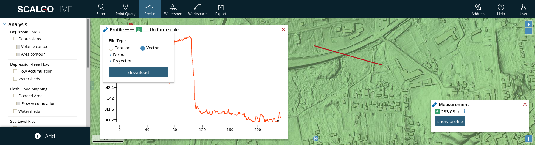
We have added the option of exporting the data in the profile window as three-dimensional polylines. For example, if you export an elevation profile you will get a polyline with the x,y coordinates following the position of the query path and z being the elevation. If you have multiple profiles in your window you will get a separate polyline for each profile. You can still choose to download the profile information in tabular form where we support CSV and the Excel spreadsheet format (xlsx).
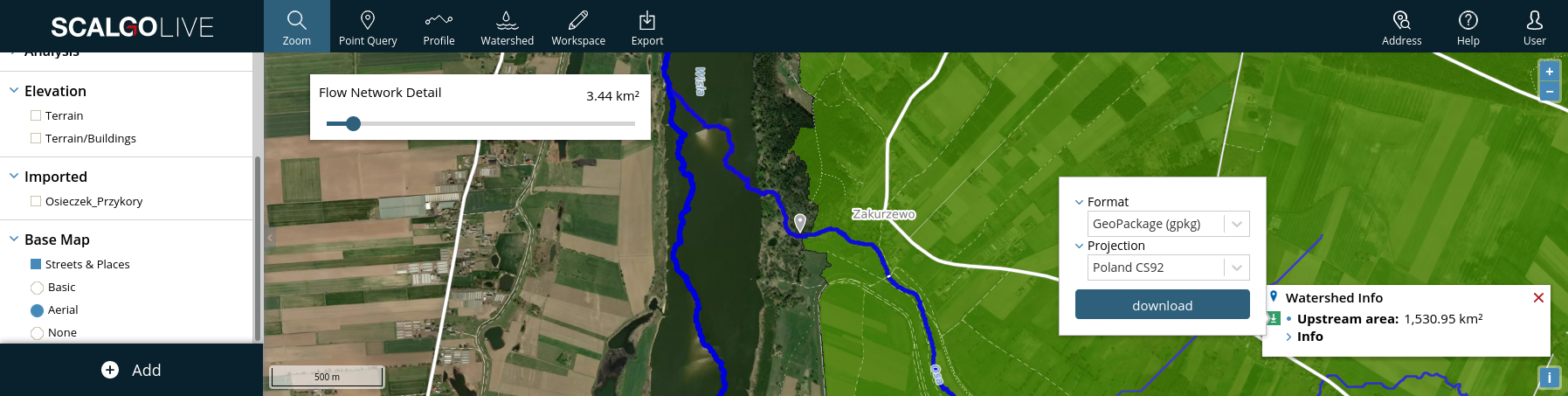
Improved download of terrain edits and query data
You can now download workspace terrain edits in the same way as you would download from other layers in SCALGO Live. First you draw a boundary around the features you want to download using the download tool, and then you click the green icon to the left of the Terrain Edits layer. You then have the option of selecting the file format and projection for the downloaded features. As part of this change the "Export features" action in the workspace menu has been removed.
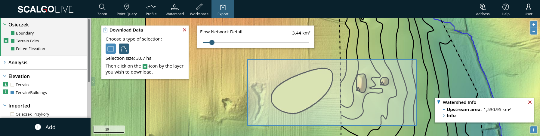
We have also added format and projection selection options for the remaining vector exports in SCALGO Live. Most notably this includes depression queries in the depression map, and watersheds exported through the watershed tool.
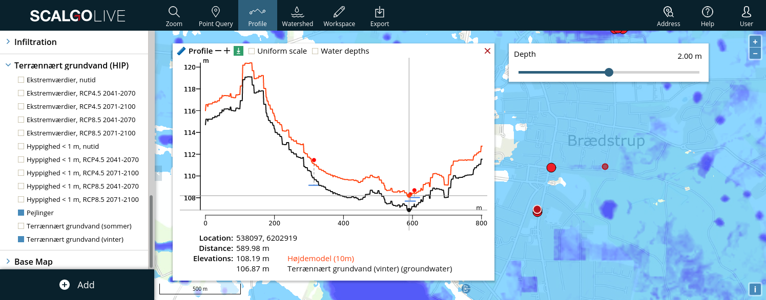
National Danish groundwater model
We have added new Danish national groundwater maps from "Hydrologisk Informations- og Prognosesystem" (HIP) in SCALGO Live. The new layers are integrated with our existing tools to create a powerful way to understand both surface water and shallow groundwater in one place. You can see the groundwater table in our profile tool and filter the groundwater maps based on depth, return period or frequencies. You can also easily understand and get information about the measurement points used the production of the HIP model.
The new layers are available from the library, and all the data can downloaded easily through our regular download system.
New Sweden high-resolution model
We released a significant upgrade to the Swedish elevation model in SCALGO Live. The new model is Lantmäteriets 1m-resolution Markhöjdmodell Nedladdning, grid 1+ which is based on Laserdata NH and Laserdata Skog. As part of this update we have also added additional corrections along rivers and longer subsurface pipes to the set of conservative corrections used in the national model. Laserdata Skog is continuously updated and thus also Markhöjdmodell Nedladdning, grid 1+ . We will regularly update the elevation model in SCALGO Live to ensure you also benefit from these updates.
We have switched the base map used for showing orthophotos and as a consequence of this, orthophotos can now be downloaded in the same way as most other layers in SCALGO Live. If you want an orthophoto for your report you might still be better off using our export map tool that will give you a georeferenced PDF that is of reasonable size.
The sea-level rise analysis has also been updated and now includes the ability to use a depth filter. The depth filter allows you to hide flooded areas where the water depth is lower than a threshold. This is now also available in workspaces.
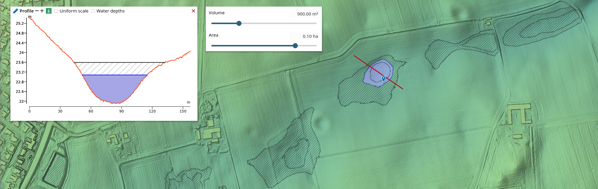
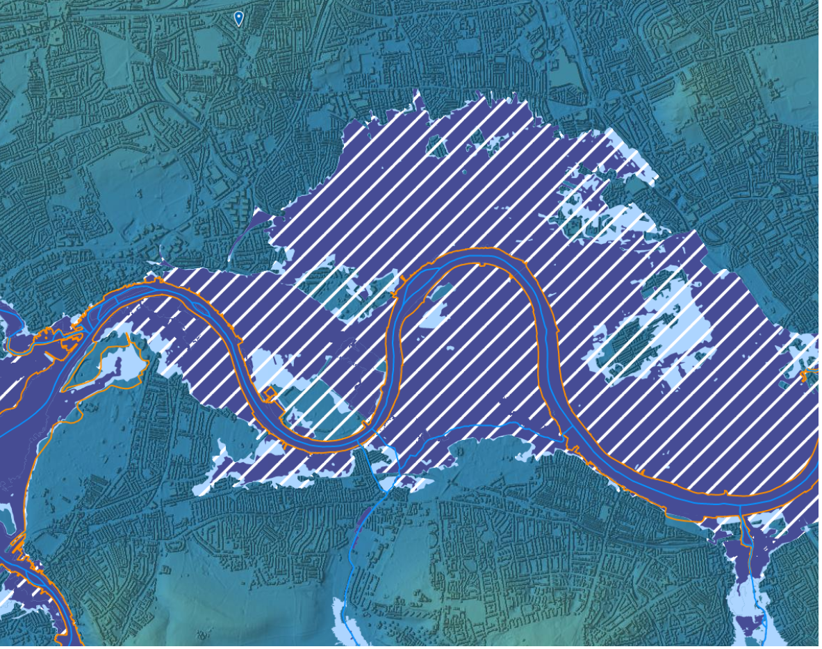
New powerful depression map and more analyses visualization options
SCALGO Live's depression map allows you to investigate the depressions in the terrain and has just become much more powerful. You can now use new volume and area sliders to hide small depressions and focus on the bigger ones. Furthermore, the default rendering style has been changed to a hatched pattern that makes it easier to distinguish between inside and outside of a depression.
But that's not all, several other interesting features have been added to the depression map:
- On point queries you now get the area of the maximal depression and the area of the selected region as well.
- You can download the map as both an area and volume raster, and as depression polygons annotated with area and volume.
- The profile tool now shows depressions too.
- A banded rendering style is now supported - more on that below. You can use either volume or area to define the bands.
- We now support volume and area contours, allowing you to easily find areas in a depression with a particular capacity.
Some of these features are shown here:
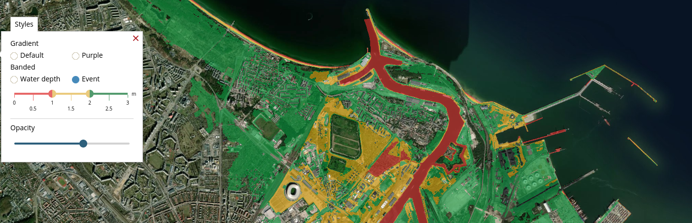
Banded styles for all analyses
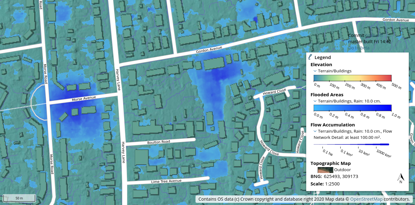
We now support banded rendering styles for all analysis layers. Banded rendering allows you to color the analysis layers in three color bands defined by two threshold values on water depth or event. Previously this was possible only for the flash flood map. Furthermore we have tweaked the colour palette to get a nicer looking output. We have also created a colorful slider to help you set the right threshold values.
Introducing Modelspaces: Get your hydrodynamic models into SCALGO Live
With SCALGO Live modelspaces you can now import your hydrodynamic models into SCALGO Live where the simulation results come to life through advanced visualisation, interactive exploration and easy sharing with colleagues, clients and consultants.
You can read more about Modelspaces on the add-on page or get the details in the documentation.
Use case videos
We have made new learning material that demonstrates how you can approach different projects based on concrete use cases. These new use-case videos cover a wide range of topics and demonstrate how the tools in SCALGO Live can be used for different purposes. The videos will give you inspiration about out what projects are possible with SCALGO Live, and provide you with guidance on how to carry them out.
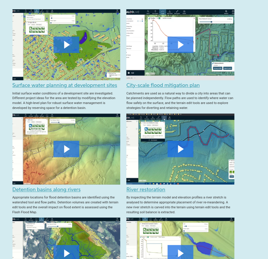
Just getting started with SCALGO Live? We also have a number of getting started videos that can help you with the basics.
Links to the use case and getting started videos are available from the Help menu inside SCALGO Live.
Access a EA flood maps inside SCALGO Live
By popular demand we have made some of the Environment Agency flood risk assessment maps and flood zone maps for England available directly in SCALGO Live.
Flood maps for planning
From the flood maps for planning service we have added the following layers:
- Areas benefiting from flood defence
- Flood defence
- Flood storage area
- Flood zone 2
- Flood zone 3
- Main rivers
Flood warning information service
From the flood warning information service we have added depth and speed layers for the low, medium and high risk rainfall scenarios corresponding to return periods of 30, 100 and 1000 years. To make this easily accessible inside SCALGO Live we have created a slider that allows you to quickly navigate between the return periods. We have also given you filters on water depth and velocity so you can focus on areas with a certain minimum water depth or velocity.
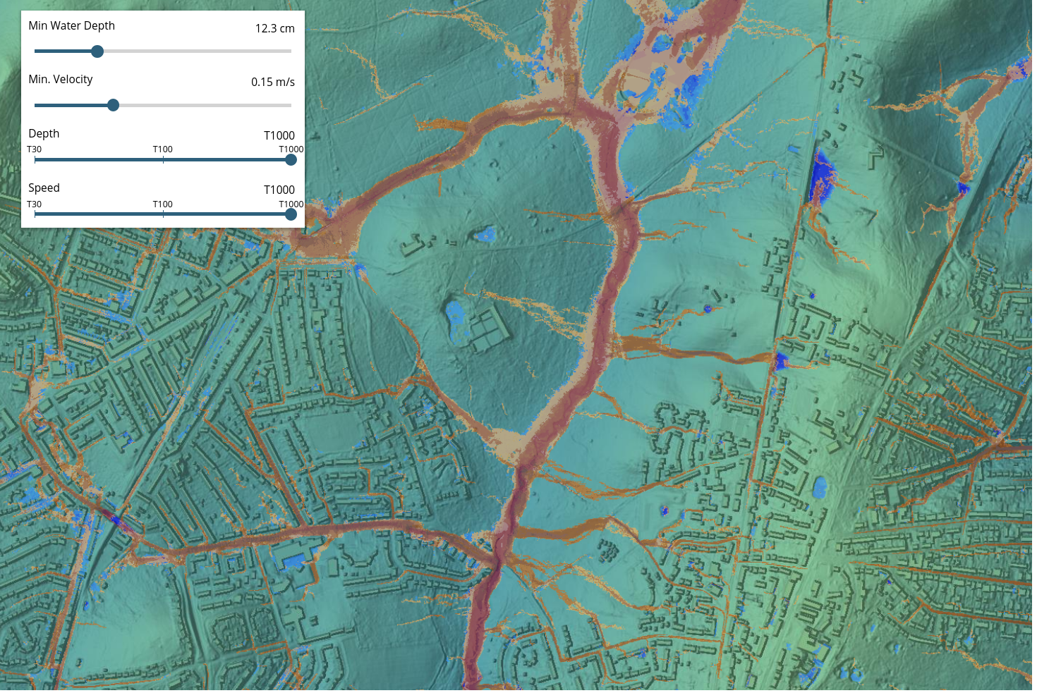
All the new layers are available from the library.
Improved map export
We have improved our system for exporting SCALGO Live maps to images as JPG and georeferenced PDFs. The new system is significantly faster than the old system and does a better job at determining an appropriate size for dialogs in the output, including the legend. By popular demand, we now also include vector data that you have dragged into SCALGO Live for visualisation in the exported document.
Try it out and don't hesitate to let us know what you think.