Streams and Flow – Computations
In this section, we describe how the stream flooding analysis works in SCALGO Live. There are two main components to the analysis:
- Computing the height of the water surface along the stream (1D-anaylsis)
- Distributing the water onto the terrain surface (2D-analysis)
Computing along the center line
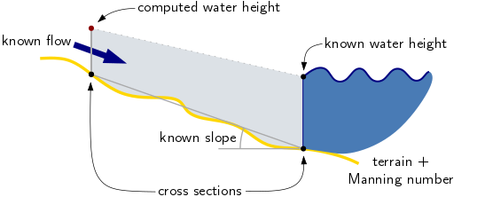
The stream network computations use the so-called Manning formula to compute the water height at each of the nodes in the open channels of the stream network. The stream network is defined from outlet points, fingertip points and in some cases a center line from the national computation. These concepts are explained in more detail for workspaces in the workspace section of this manual.
Once the network has been defined, we use it to query the elevation model to create cross sections at fixed intervals. We do not create cross sections on subsurface structures, e.g., when the stream goes underneath a bridge or through a pipe.
Following the cross section sampling process, we have a stream network with nodes and channels with cross sections. This is the starting point of the Manning-based computation. The computation proceeds upstream from the outlets of the stream network. At each step, the water height is computed based on the previously computed (downstream) water height, the slope of the edge connecting the two nodes, the cross section information, the flow values and the Manning number.
The water flows on the surface of the terrain and the flow is modeled in a steady-state where all flow passing into an edge in the network also passes out of it. There is no water storage intern to the network. As such, the model is stationary and does not provide a time-dependent estimate of the flood risk.
Note that we only support flow in open channels. If you have a subsurface structure (such as a bridge or culvert) in your network the water level will be forwarded unchanged from the downstream to the upstream point. This is also the case for the national analysis.
Water on terrain
The next step after computing the elevation for water level along the stream network lines is to show what parts of the terrain adjacent to the stream is at risk of flooding. When flooding the terrain we follow the flow paths backwards (upstream) from each point on the stream. We mark the cells on this path flooded until the cell elevation is higher than the elevation computed on the network line. This is illustrated below:
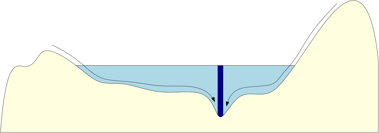
Consider a location on the terrain, away from the stream, with an elevation of 20 meters. Let us assume that this location has a downstream flow path to some location on a stream. The cell is then flooded if the elevation of the water level in the stream at that particular location is 20 meters or more. This method is easy to understand and effective, one of its benefits is that the flooding can follow the terrain and reach locations without direct line-of-sight to the stream.
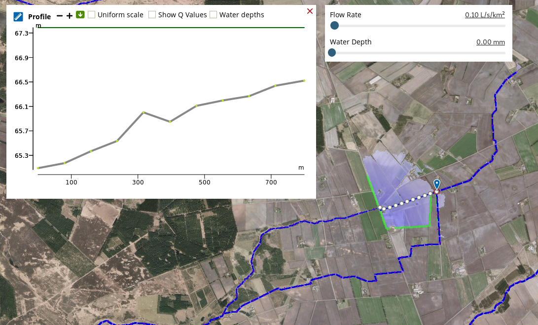
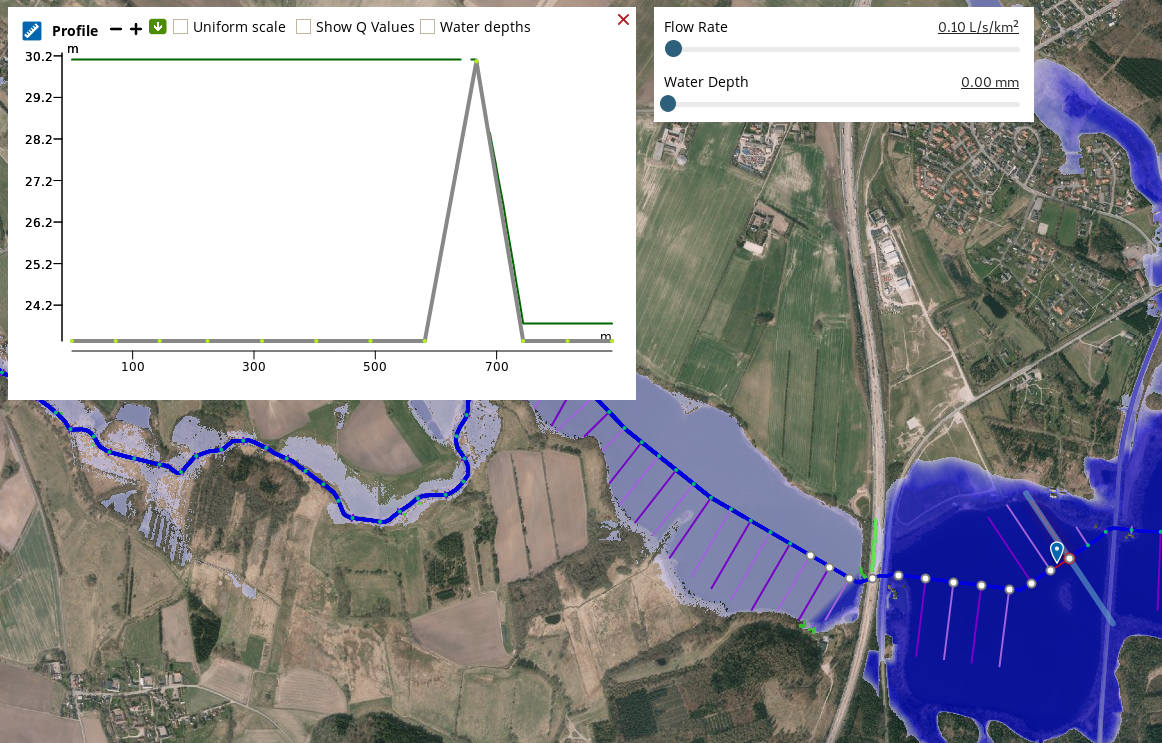
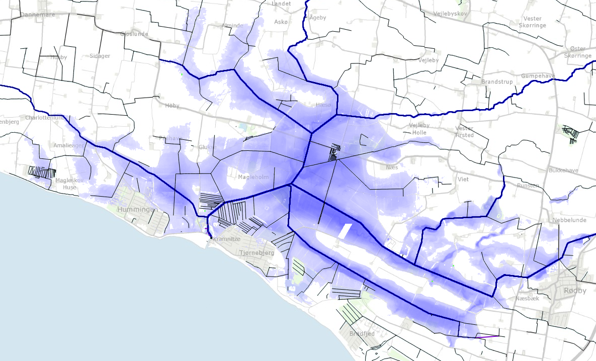
A fundamental property of this method is that the water level of any location of on the stream only affects cells in the watershed of that cell. The figure below shows an example flooding event seen from above.
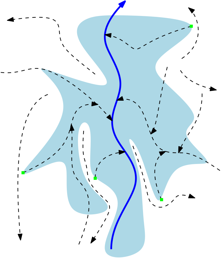
To understand what parts of the stream affects what part of the terrain you can use the subwatersheds layer to see what sections of the stream each location in the terrain drains to.
Indirect Flooding
Since a location in the terrain is only marked as flooded if its elevation is lower than the water level of the part of the stream into which it drains.However, it is still possible for the water to reach other parts of the terrain and in fact, the flooded areas can have a surprising boundary simply due to theterrain watersheds. The picture below shown an illustration:
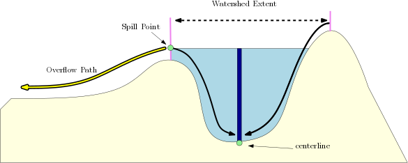
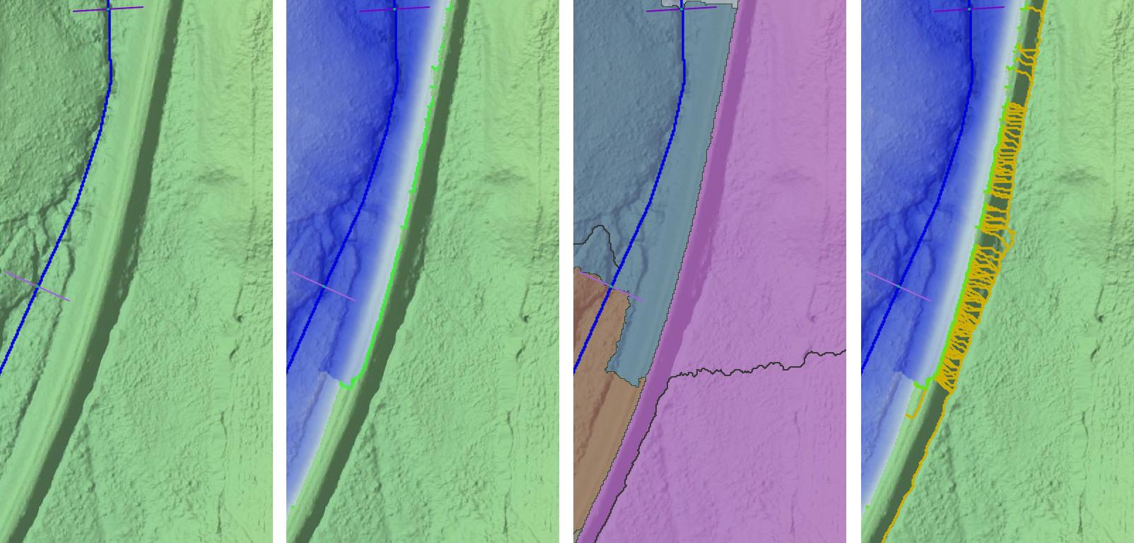
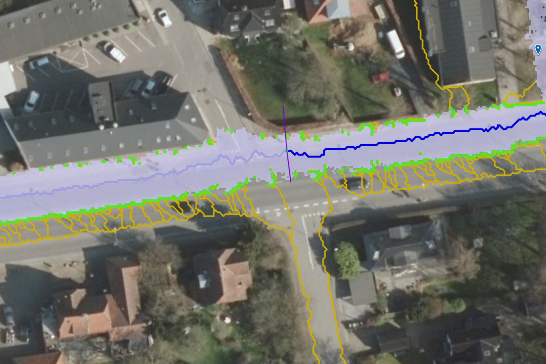
At the spill point in the figure above, the flooding extent stops at a location with non-zero water depth. In practice you would expect some flooding on the side of this spill point due to the water overflowing at the watershed boundary on which it lies. We use the term indirect flooding to refer to the regions that are at risk of flooding but are not shown as such due to the way the flood-method operates. To investigate the risk of indirect flooding we display so-called overflow paths which captures the overflowing mentioned before. The overflow path shows what happens when water spill over at watershed boundaries and continue downstream just like any other flow path in SCALGO Live.
An example of this is shown in the series of screenshots below where we investigate an extreme flooding event in a stream running parallel to a roadway.
Overflow paths and indirect flooding is not only important on streams. When
looking at flow across arbitrary flow paths they become a powerful tool for
understanding what happens when certain flood thresholds are met
The national analysis: Notes and caveats
GeoDanmark streams are annotated with a synlig attribute meant to signal if the stream is visible in an orthophoto or not. We use this field to decide if a section of the stream is running in a pipe, underpath or similar closed-channel. The computation simply forwards the waterlevel across this area.
We use a constant Manning number of 24 in all streams nationwide.
The national analysis is based on combining the Danish Elevation Model with GeoDanmark data and models roughly 10.000 kilometers of streams. Due to the different data sources, properties of the elevation model and the hydrological model, there is a number of known issues that can appear in the national analysis. We list these below along with suggestions for how these issues can be mitigated if your study area happens to exhibit one or more of them.
Flood risk screening on the elevation model
Typically national elevation models like the ones used in SCALGO Live does not show information about the bottom of streams and rivers. The model usually reflects the water level at the acquisition time since the scanner used does not penetrate the water. Thus one often makes the assumption that the elevation in the model reflects some known "basis"-flow, assuming the acquisition was made on a day where the flow in the streams were normal for the period. If the basis flow is Qbasis and you want to model a 100 year event with flow QT100 then you simply subtract Qbasis from QT100 to get the flow to use in the analysis.
When the stream is close to the ocean and the bottom elevation of the stream is less than the sea-level the cross section profiles of the streams are partly filled with water from the sea. This means that Qbasis alone does not explain the water level in the elevation model. Thus you have to be careful selecting the right flow value in these situations.
Breaking cycles in the GeoDanmark center line
We do not support branches in the downstream direction in our hydrological model, e.g. a stream splitting in to. In fact, we require that each stream only has one possible path to its outlet (typically the ocean). Thus, in cases where there is a split in the stream network, or some other cyclic structure in the network, we break it up by removing a segment in the center line. This is done using a heuristic and sometimes makes choices that are not ideal and can cause the direction of flow to reverse direction such that the flow goes uphill. Our stationary Manning-computation cannot model a decrease in water level in the upstream direction and this can cause a large amount of local flooding in the model.
Mitigation: Since the stream network is flawed in this location you will not get a different result by creating a stream workspace based on the national computation. However, you can create a regular workspace and enable the stream network analysis. You can then use the regular flow directions in the elevation model to model this stretch of the stream.
Incorrectly marked bridges
If the stream line in GeoDanmark is not correctly marked as not visible when it goes through a bridge it will appear as if the bottom of the stream "jumps" up to height of the bridge and then goes down again on the other side of the bridge. This acts as a big barrier in the stream and causes the water level upstream of the bridge to the elevation of the top of the bridge, causing potentially large areas to be flooded. This is not a common problem, but when it does happen it can have significant effects as evidenced in the example below.
Mitigation: You can simply create a workspace of that same area and lower the elevation of the bridge to fix the issue. Note that in the example above your workspace should contain the whole of the flat lake to get the boundary conditions right. We refer to the workspace section for more information.
Pumped areas
Our hydrological model does not model the function of pump stations along the stream and this causes problems for places behind a pump station. These places are typically lower-lying than the area downstream of the pump and the Manning-computation will model the steady state as if the pump did not exist. This causes the area normally protected by the pump to be flooded by the stream at the water level it has downstream of the pump station. These places are relatively easily identified in the analysis as large flooded areas of low elevation relative to the elevation of the streams draining out from them.
Mitigation:
If you want to model an area behind a pump - or a workspace that includes a pump, you can do so in workspaces. If your workspace contains a pump so you can use an event point to "reset" the water level upstream of the pump to an appropriate value. If you want to model that a certain volume of water is behind the pump you can use the depression map to figure out how much terrain would be flooded by that amount of water.