Modelspaces – Introduction and Use

Scalgo Live supports importing, visualizing, and sharing results from hydrodynamic model simulations, including time-series data, through hydrodynamic modelspaces.

Creating modelspaces

To create a modelspace you can follow these steps:

1. Go to the Library.
2. Click the Modelspaces tab, and click Create new modelspace.
   
3. Select a file to open.
4. Check the spatial reference if necessary.
5. Choose the layers, and their types, from the file you want imported into Scalgo Live.
6. Click import.

When importing large files, remember to use a computer with a fast and stable internet connection, if the process is interrupted it has to be restarted. Once the modelspace is created, you can of course use any computer you would normally use for Scalgo Live to interact with the results.

Selecting layer types

In step 5 of the modelspace creation process you tell the system how to map the data in the file to the types of data supported in a Scalgo Live modelspace. Currently the 5 basic types supported are:

• Elevation data
• Absolute or directional flux
• Absolute or directional velocity
• Water depth (relative)
• Water level (absolute)

The system will try to detect what type the data in your file corresponds to, but this is not always possible and you can therefore tweak it. Here is an example of this process inside Scalgo Live:

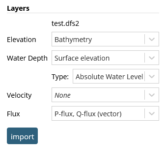
On the left side we show the different types supported by Scalgo Live and on the right side the layers from the file that will be used for each type is shown. If you want a different layer to be used, or do not want to import a given type at all, you can use the drop-down box to change the selection.

Adding and removing data

If the output of your simulation is stored in multiple files covering the same area, use one to create the modelspace, and then click Add or replace layers... in the modelspace dialog to import each of the remaining files.

To remove superfluous layers, simply click the trash can showing next to the layer name while hovering your mouse.

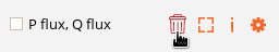
Layer removal is permanent, if you change your mind you will have to re-upload the data to the modelspace.

Events

Results from simulations of different events on the same model can be grouped into one modelspace by selecting New event when uploading the result, and then using Add or replace layers... to upload the remaining results.

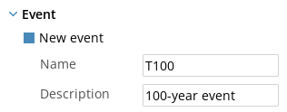
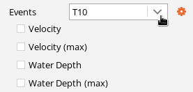
Results associated to events are then found under the Events header in the dock.

Note that the elevation layer is shared between events.

Time-series data

If the input data represents a time-series of steps in a simulation run, both the individual time steps as well as the maximum value over all time steps can be visualized. A time-slider is presented to browse through the steps of the simulation. The time shown is relative to the start of the simulation.

Use the play button (▶) to watch your simulation as a video. The playback speed factor (relative to the simulation time), is shown and can be changed by clicking it repeatedly. The choice of speed factors depends on the simulation time step and duration.

Hydrodynamic data types, visualization and interaction

Flux & Velocity

For flux and velocity we support vector fields, typically represented by an x- and y-component or absolute value and angle. If two components are present in the input data, they will be combined into a single layer, with the option of showing the data using a gradient where the colour depends on the absolute value (Euclidean norm) of the two components, or using arrows showing the direction. The size of the arrows again depends on the absolute value of the vector. Velocity data can also be visualized using a particle animation (see below for details). If the data is represented as one component, this is assumed to be the absolute flux or velocity, and only the gradient visualization is available.

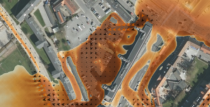
Velocity layers with two components can be visualized with animated particles. The particles are placed randomly on the screen and displaced by the velocity vector at their current location on every animation frame. Fading lines connect particle locations over time, creating an intuitive animation of the modelled water flow. Currently there are three animation styles available to choose from:

• Animated gradient. Particles are coloured with a dark purple to light orange gradient, representing the absolute velocity. The colour scaling automatically adjusts to match the minimum and maximum velocities visible on the screen. This style is designed to stand out against almost any background.
• Animated white. Particles are semi-transparent, enabling simultaneous viewing of other layers alongside the velocity animation. Choose this style if you need to overlay velocity information with other data.
• Animated particles. This style displays a reduced number of white particle traces. It is especially suitable for overlaying on water depth or flux, allowing you to clearly see the background while analyzing flow patterns in detail.

These visualisation styles will give you a feel for the relative velocities in a simulation. By combining different Modelspace layers, you can spot high-flux areas with critical water depths and fast flows.

Note that the behaviour of the threshold slider for flux and velocity layers differs depending on the selected visualization style:

• When using arrow visualization, the slider is used to control the maximum flux or velocity. Arrows representing values larger than this maximum are drawn in red.
• When using gradient visualization or particle animation, the slider is used to control the minimum flux or velocity shown.

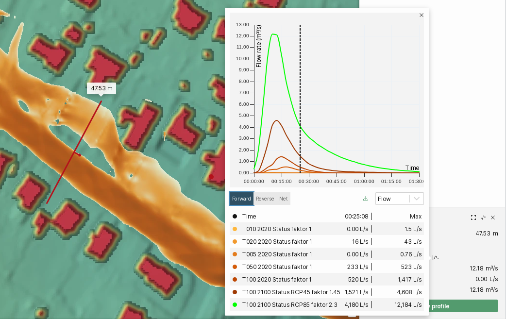
To analyze flow and volume across a line, use the profile tool while you have a flux layer enabled. Water can flow from either side of the profile line to the other side. We refer to these two flow directions as the forward and the reverse direction. The forward direction is indicated with a small arrow on the profile line. With the profile tool, you can measure the flow and the volume for both directions, as well as net values, at the selected time. Click the graph icon next to the flow value to get a graph of flow and volume over time for all events.

Please note that the accuracy of the computed values depends on how well flow is sampled over time: if e.g. peak flow occurs right between two time steps, the computed flow (and volume) may be lower than when the peak would be sampled accurately.

Point queries on layers with direction return both the absolute flux or velocity and the compass direction (azimuth) with respect to grid north in the visualization projection.

Water depth & Water level

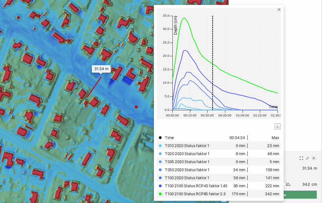
Water depth data is displayed similarly to the water-depth visualization for the flash-flood map and sea-level rise, with a default blue gradient and the option of "banded" visualization. If you enable the profile tool and draw a line, the maximum water depth along the line is shown, and by clicking the graph icon, you can see the water depth over time, for all events. The graph is also available for point queries.

Water depth layers are also rendered in the profile window, and update with the time slider.

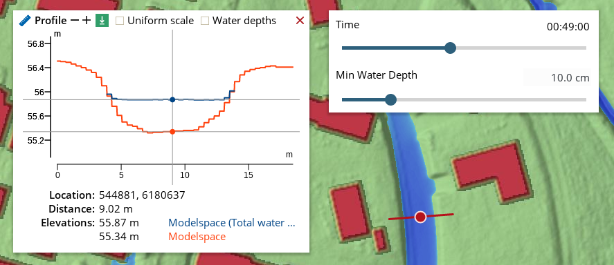
During import, water level data is converted to water depth by subtracting heights from the supplied elevation model.

Note that the absolute water level displayed in the profile window is the result of offsetting the water depths on top of the terrain model. If the terrain model is resulting from the interpolation of mesh vertex elevations, the water level may not appear flat when the terrain is sloping. For some input file formats one can use an elevation model based only on the elevations at the center of the mesh elements, which results in a much less pleasing visualization of the terrain model where all mesh elements are level, but on the upside, the profile window will then show the water levels being flat.

Computing flux

If your modelspace contains velocity and water depth data, but is missing flux layers (as is common for the output of some modelling packages), you can click Compute flux in the modelspace dialog to compute flux (both time series and max flux) from velocity and water depth. This simply multiplies the water depth and velocity in each cell, and allows you to visualize flux as well as use the profile tool to analyze flow through a cross section.

Sharing modelspaces

Modelspaces can be shared with other users of Scalgo Live in the same way as workspaces.

Additional layers

If you select an elevation model for your modelspace, Scalgo Live will automatically compute additional analyses based on this model for your convenience. Currently we compute the depression map, which is available as a layer in the modelspace, and we enable the watershed tool allowing you to dynamically query (depression-free) watersheds in your elevation model.

For modelspaces created through DynamicFlood, additional layers are available containing the terrain edits, objects, and buildings in the simulation. The layers are copied from the workspace at the time of starting the DynamicFlood simulation.

Note that for modelspaces created from uploaded data, meshes are rasterized upon import and the analyses are computed on this rasterized model.