Country Specific – Germany

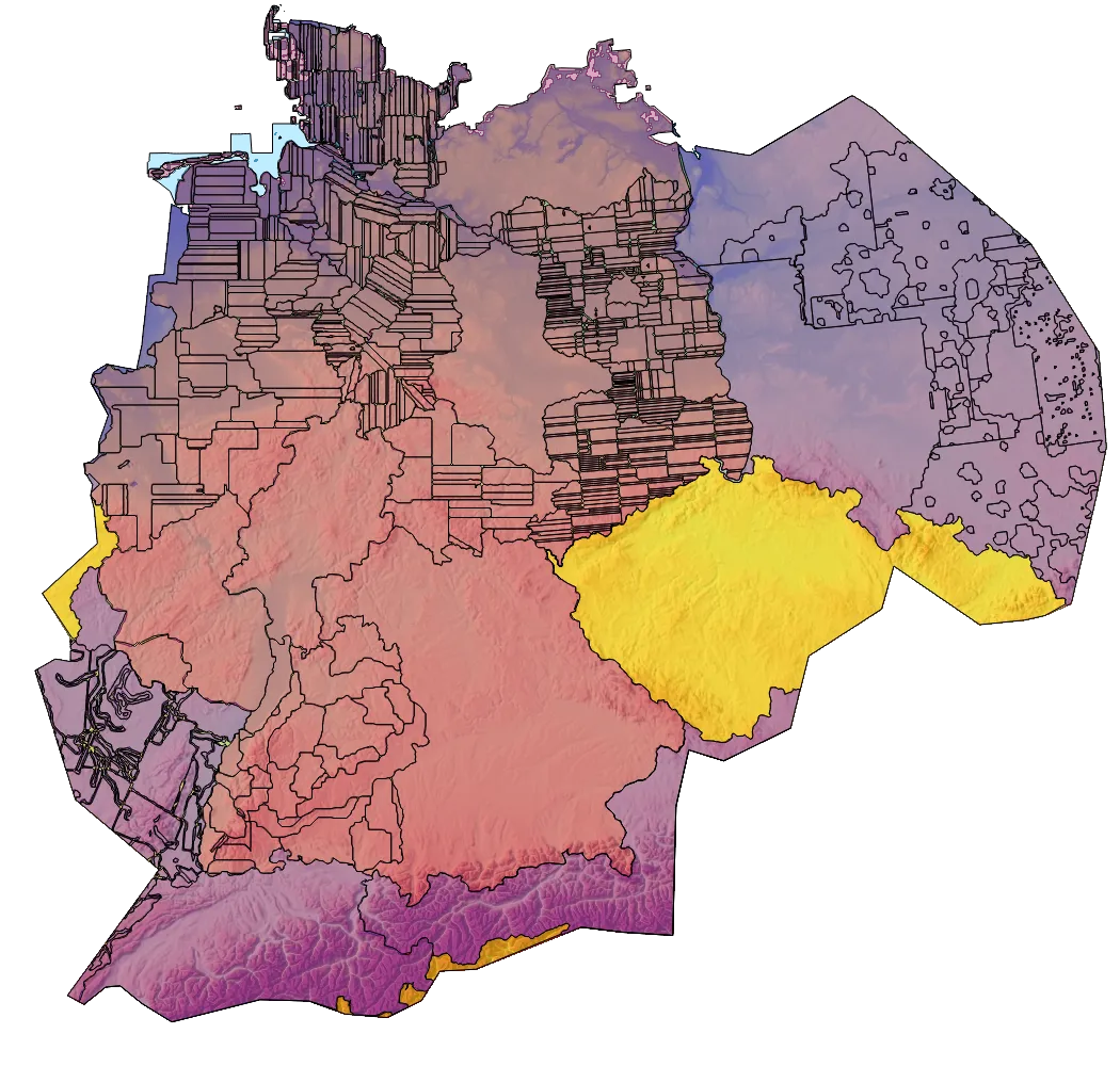
The elevation model for Germany in SCALGO Live is based primarily on the states DGM1 with fallback to DGM2 or BKG's DGM5 where these are not available as open data.

• Bayern: DGM1
• Baden-Württemberg: DGM1
• Berlin: DGM1
• Brandenburg: DGM1
• Bremen: DGM1
• Hamburg: DGM 1
• Hessen: DGM1
• Mecklenburg-Vorpommern: DGM1
• Niedersachsen: DGM1
• Nordrhein-Westfalen: DGM1
• Rheinland-Pfalz: DGM1
• Sachsen: DGM1
• Sachsen-Anhalt: DGM2
• Saarland: DGM1
• Schleswig-Holstein: DGM1
• Thüringen: DGM1

To accommodate resolutions down to 1 m, all analyses are done in 1 m resolution for the whole country in ETRS89/UTM32.   The vertical reference used is DHHN92.  Workspaces constructed from this model also have a resolution of 1 m. We strive to keep the model up to date with the latest sources.

In order to use an elevation model for hydrological analysis of surface water, such as watershed and flow accumulation computations, three conditions need to be met:

• The upstream area of any river should be covered by the elevation model.
• Structures on top of the terrain should only be present in case they actually block water from flowing under or through them.
• Structures transferring water below the terrain surface should be taken into account.

Below, we discuss how we process the model to fulfil these conditions as well as possible.

Extensions

In order to cover the upstream areas of all rivers crossing the country, we have extended the model in the following areas:

• For Switzerland, contributing almost entirely to the Rhein, we use the 0.5 m swissALTI3D model (resampled to 1 m) from the Federal Office of Topography swisstopo.
• For Austria's contribution to the Donau, we use the 10 m Digitales Geländemodell Österreich.
• For Poland's contribution to the Oder, we use the 1 m Digital Terrain Model made available by the Head Office of Geodesy and Cartography (GUGiK).
• For France's contribution to the Mosel and Rhein, we use the 1 m RGE Alti model.
• To cover minor streams on the border with Denmark, we use the 0.4 m Danish elevation model (DHM) (resampled to 1 m) produced by the Danish Agency for Data Supply and Infrastructure (SDFI).
• Similarly for the Netherlands, we use the 0.5 m Dutch elevation model AHN4 (resampled to 1 m).
• For Luxembourg's contribution to the Mosel, we use the 0.5 m MNT LiDAR 2019.
• To cover remaining areas of the Czech Republic, France, Luxemburg and the Netherlands that contribute to flow in Germany, we included data from the 30-meter EU-DEM data set, which in turn is based on SRTM and ASTER GDEM data.
  

A full overview of which data source is used for which part of the model is available by clicking the gear icon next to an elevation layer, selecting the "Source" tab, and "Show source information". Use point query to see more details for individual areas. Multiple styles are available for this layer to colour sources by e.g. date and resolution.

Buildings

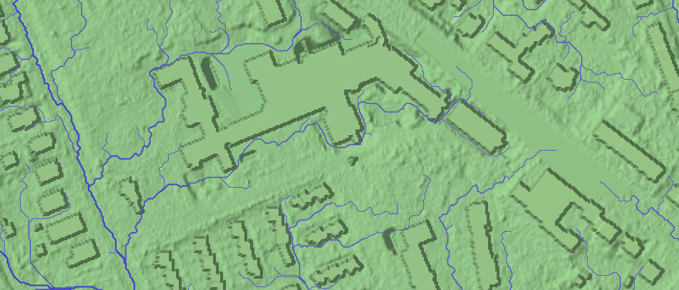
Buildings are not included in the terrain models, since they represent the "bare earth" elevations. When computing water flow paths, more realistic results are generally obtained when the elevation model does include buildings so water can be simulated to flow around them. In SCALGO Live, we accomplish this by adding buildings back into the model using a data set of building footprints, where we raise all grid cells covered by a building to a height 10 meters above the highest terrain point within the building footprint. This model is called "Terrain/Buildings" and is the basis for all nationwide hydrological computations.

The building footprints are taken from the AdV Hausumringe Deutschland (HU-DE) dataset, but exclude footprints of bridges, sluices, weirs, etc.

Bridges, underpasses and hydrological corrections

Major bridges have generally been removed from the models, but for many smaller bridges and underpasses additional hydrological corrections that allow water to flow through such structures are necessary. SCALGO Live Germany includes a nationwide hydrological correction set based primarily on the Basis-DLM data from BKG. Corrections have been generated at intersections between buildings and rivers lines, and river sections marked with the "HDU_X" property, indicating the river is flowing under something. Each correction thus follows a line in the river network, with end points adjusted to match the elevation model as well as possible.

The set of corrections is available under the Hydrological Corrections category in the Library.

The national analyses use these corrections, and workspaces created using the predefined "Flash Flood Map" or "Sea-Level Rise" buttons also include them by default. If you create a workspace through any other means than the predefined buttons (e.g. if you upload your own model), you can include corrections in that workspace through the workspace Actions tab by clicking Import corrections; they will not be included automatically.

Land cover

The land cover map in SCALGO Live is produced by SCALGO based on machine learning techniques at a resolution of 20 cm. It is available as a standalone layer in the Land Cover category in the library.

The land cover map segments the country into 11 different classes. When downloaded as a raster, the categories have the following numerical encoding: 1 for bare land, 2 for water, 3 for other paved, 4 for snow or ice, 6 for shallow vegetation, 7 for dense vegetation, 8 for farmland, 9 for paved road, 10 for unpaved road, 12 for railroad, 15 for bare rock, and 16 for building.

Watershed queries

When you perform a watershed query you can see the land cover distribution of the watershed.

Annotated administrative regions

We have annotated a number of datasets, including the cadastral parcels (ALKIS Flurstücke, see below) and administrative regions with information about land cover. You can find those layers in the Land Cover category alongside the land cover map itself. For each region in those data sets we have added a field that provides the total artificial area in the region, as well as the ratio of natural to artificial in the region.

ALKIS cadastral parcels (Flurstücke)

We have aggregated cadastral parcel information from the below federal states into a single layer called Flurstücke under the ALKIS category.

• Baden-Württemberg
• Berlin
• Brandenburg
• Bremen
• Hamburg
• Hessen
• Mecklenburg-Vorpommern
• Niedersachsen
• Nordrhein-Westfalen
• Saarland
• Sachsen
  
• Sachsen-Anhalt
• Schleswig-Holstein
• Thüringen

Soil type

The soil type data used in SCALGO Live Germany is based on the Geologische Übersichtskarte der Bundesrepublik Deutschland 1:250.000 (GÜK250) from BGR.  Specifically, we use the Basislayer and Überlagerungslayer Petrographie, and map the BGR classes to SCALGO soil types according to this table.  For more information about the SCALGO soil type classes as well as how we produce the topsoil map, see the soil type documentation.

The following relevant layers are available in the Library:

• The original layers published by BGR can be found in the BGR (wms) category
• The result of combining the BGR layers and mapping to SCALGO soil types can be found in the BGR category, layer BGR GÜK250 soil types.
• The topsoil map can be found in the BGR category, layer Topsoil type.
• The urban polygons used for the topsoil map can be found in the Land Cover category, layer Stadtgebiete.  See the layer description of this layer for more information on how it was constructed.

Rain

Design rain events in Germany are based on the KOSTRA-DWD-2020 dataset provided by the Deutscher Wetterdienst (Junghänel, 2022). The dataset provides parameters for analytical IDF curves on a 5x5 km grid for the whole country. We create design rain events from these parameters using the methodology described in the Chicago Design Storm section with the only difference being that parameter a is estimated from the return period and is defined by (Junghänel et al., 2023):

Where T is the return period in years and ξ, β, and κ are parameters from the generalized extreme value distribution (representing the location parameter, scale parameter and shape parameter respectively).

A layer showing the gridded rain regions is available in the library under Rain.